Creating a pivot table in Excel or Google Drive is not as difficult a task as it sounds. The feature allows you to visualize and summarize data from tables without having to use any formula! That is, it is very useful for those who do not have much practice with spreadsheets.
teaches you how to create pivot tables in these two editors and make your life easier. Check out!
How to Create a PivotTable in Excel
To create a pivot table in Excel, you must have at least the 2022 version of the program. Previous editions do not have this feature.
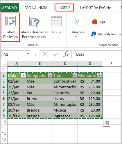
1. Open the Excel document with the table you want to transform into a pivot table;
2. Select the table snippet you want to include in the pivot table. To do this, click on the first cell, hold down Shift pressed and click on the last cell of the table. If you want to select independent cells, hold down Ctrl pressed while clicking on the cells;
3. Then in the tab Insert, patch me Dynamic table;
4. In the window that opens, perform the following actions:
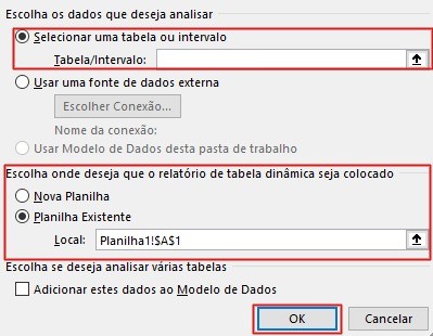
- Check the option Select a table or range;
- just below, in Table/Range, confirm that the selected cell range is correct. It is normally displayed automatically;
- Em Choose where you want the PivotTable report to be positioned, opt for New Worksheet, in case you want to create the table on a different worksheet. Or, choose Existing Worksheet and select, with the mouse, the area where you want to insert it;
- Complete the process in OK;
5. Now it's time to configure your table. In the right sidebar, check the fields (columns) you want to include in the pivot table. You can combine the fields or view the data for each one individually. The table changes automatically;
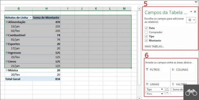
6. Just below, note that it is possible to drag the fields between filters, columns, rows and values;
7. By default, the pivot table displays the sum of the displayed values. If you want to change the operation, go to Sum of Amount and then in Value field settings;
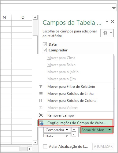
8. In the window that opens, select whether you want the average, maximum, minimum, product, and other options to be displayed. confirm in OK.
20 tips for those who know nothing about Excel and want to learn the basics.
How to create a pivot table in Google Drive Sheets
To perform the procedure below, you must have a Google account or that a user has shared a spreadsheet of the service with you.
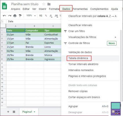
1. Open the Google Drive spreadsheet with the table for which you want to create a pivot table;
2. Select the table cells you want to include in the pivot table. To do this, click on the first cell, hold down Shift pressed and click on the last cell of the table. If you want to select independent cells, hold down Ctrl pressed;
3. Please click DATA, at the top of the screen, and choose Dynamic table;
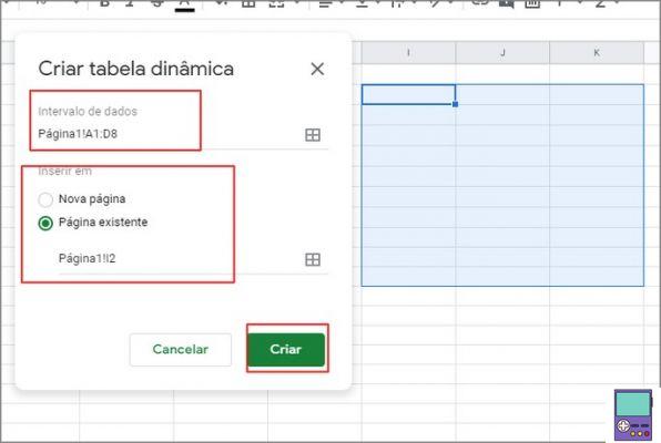
4. In the window that opens, check if the chosen data range is correct. just below, in Insert em, opt for New page, if you want to create the pivot table in a new tab. If you prefer it to be inserted in the same tab, choose existing page. Then, select the cells where it will be applied and confirm in Create;
5. In the side column, you must choose which content of the pivot table you want to view. To do this, click Add to Cart, beside Lines ou Columns. Then select the fields to be displayed. You can combine the fields or view the data for each one individually. The table changes automatically;
6. If you want to change the displayed operation, go to Values and click Add to Cart. Then choose the value you want to see in the rows or columns. It can be sum, product, maximum, minimum, average, among other options.
What is a pivot table and what is it for?
The pivot table makes it easy to visualize and interpret data. There is no minimum number of rows or columns to make a pivot table. But the tool is perfect for generating summaries of large spreadsheets.
According to Microsoft, the tool allows you to calculate, summarize and analyze information. With this, it facilitates the visualization of comparisons, patterns and trends in real time. You can, for example, move rows and columns, filter information, restrict data from a set, and much more.
Tips for making a pivot table
If, by chance, you tried to transform a table into a pivot table and you couldn't, it is possible that you made some "error". That's because, to be successful, it is necessary to follow some simple but fundamental rules.
- The data must be in table format and empty rows or columns are not allowed;
- The data types in a column must be the same. That is, it is not possible to create a pivot table if the column contains dates and prices, for example;
- Each column must have a header;
- In Excel pivot table, columns are called Add more. According to Microsoft, this is because it is a traditional term used in database and data applications;
- In the case of Drive, the pivot table feature is not available in the Android and iOS apps, only in the desktop version.
recommends:
- 30 Excel formulas to master spreadsheets
- Discover apps that can help you make money